For one centrifugal pump on similar operating points, flow changes with speed, head with speed squared and shaft power with speed cubed. At 80% speed, a pump that takes 30 kW at the shaft needs 15.36 kW. That result holds on a closed heating or chilled water loop, where friction is nearly all of the head. Where the pump lifts water or fills a pressurised vessel, part of the head does not fall with speed, and the saving is smaller. The third example works through one such case.
Flow
Q2 = Q1 × (N2 ÷ N1)
N is the speed in rpm, or the drive frequency. Only the ratio matters, so the unit cancels, and flow comes out in the unit you enter. Frequency is a close stand-in for speed. On a 4-pole motor with 2% full-load slip, 45 Hz gives a true speed ratio of about 0.902, not 0.9, because slip falls with the load. That moves the power result by about 0.6%.
Head
H2 = H1 × (N2 ÷ N1)²
Head, or pressure, falls with the square of speed. At 80% speed the pump develops 64% of its head, and that includes its shut-off head at zero flow.
Power
P2 = P1 × (N2 ÷ N1)³
Shaft power falls with the cube: 80% speed needs 51.2% of the power. Electrical input is shaft power plus the motor and drive losses. A drive typically runs at 97% or better at full load, and both drive and motor lose a larger share at light load, so the saving at the meter is a little smaller than the shaft figure.
The laws are exact only when the system curve passes through zero head at zero flow. A closed loop with no control valve movement meets that condition. Static lift, a pressurised receiver or a pump held at a fixed differential pressure adds head that does not fall with speed. The duty point then moves to where the pump curve at the new speed crosses the system curve, and flow drops faster than speed. Plot both curves to find it.
Pump affinity law examples
Circulating pump from 1,500 to 1,200 rpm
Check the inputs first. 200 m³/h at 40 m is 21.8 kW of hydraulic power, so 30 kW at the shaft means a pump efficiency of 73%, which is plausible. At a speed ratio of 0.8 the pump delivers 160 m³/h at 25.6 m, and shaft power falls to 30 × 0.8³ = 15.36 kW. Over 6,000 hours a year that is about 88,000 kWh less shaft energy, provided 160 m³/h still meets the load.
The loop is designed for a 6 K difference between flow and return, but it runs at 5.4 K at full load. The pump moves 120 m³/h where the coils need 108 m³/h. At 45 Hz, a speed ratio of 0.9, flow falls to 108 m³/h, head to 20.25 m and shaft power from 11 kW to 8.019 kW, 27% less. At the same cooling load, the temperature difference returns to 6 K.
If a balancing valve at the pump is throttled hard, open it as you slow the pump. The valve then stops burning head, and the pump can run slower still for the same 108 m³/h. That saving is larger than the calculator shows, because the system curve itself has moved.
A pump lifts water 25 m to a tank and delivers 100 m³/h at 40 m, so 15 m is friction. It has a shut-off head of 52 m and takes 15 kW at the shaft. At 80% speed the calculator gives 80 m³/h at 25.6 m and 7.68 kW. The system cannot run there: at 80 m³/h it needs 25 + 15 × 0.8² = 34.6 m.
The real duty point is where the slowed pump curve, 33.3 m at shut-off, meets the system curve. That is about 55 m³/h at 29.6 m, or 4.5 kW of hydraulic power. The pump is now well left of its best efficiency point. If its efficiency drops from 73% to 65%, it takes about 6.9 kW, or 0.125 kWh per m³ against 0.150 kWh per m³ at full speed. The saving per cubic metre is about 17%, not the 36% the cube law suggests. Below 69% speed, the square root of 25 ÷ 52, the pump cannot reach the tank at all.
Why is the measured saving smaller than the calculator’s?
Static head is the usual cause, as the third example shows. Control is the next. A pump held at a fixed differential pressure behaves as if that setpoint were static head, so a 20% cut in flow does not give a 49% cut in power. Moving the sensor to the index circuit, or resetting the setpoint as valves close, recovers most of the difference. Motor and drive losses take the rest, and both grow as a share of input at light load.
How far can I slow a pump down?
Static head sets a hard floor. Shut-off head falls with the square of speed, so a pump with 52 m at shut-off stops delivering into 25 m of lift below 69% speed. Above that floor, the pump manufacturer states a minimum continuous flow to limit recirculation, heating and vibration. Motor cooling is rarely the limit on a centrifugal pump, because the load torque falls with the square of speed. Set the drive’s minimum frequency to the highest of these limits.
Do the affinity laws apply to fans?
Yes. Centrifugal fans follow the same three laws, with pressure in place of head. Pressure and power also scale with air density. Air at 0 °C is about 11% denser than air at 30 °C, so correct for temperature before you compare winter and summer readings.
Can I use them for an impeller trim?
Only as a first estimate. Trimming changes the pump’s geometry, so the relationships are approximate and hold only for small trims. Use the manufacturer’s curves for the trimmed diameter.
How do I confirm the saving after fitting a drive?
Log electrical input, flow and differential pressure at 15-minute intervals for a few weeks before and after the change. Compare kW at matched flow, or kWh per m³ over weeks with a similar load. A single spot reading on each side measures two different duties. See pump performance monitoring.
Limits of this result
Where static lift dominates, do not use the cube law alone: plot the system curve against the pump curve at the new speed.
This does not check minimum flow, cavitation (NPSH), motor and drive limits or control valves.
For a trimmed impeller or a viscous fluid, use the manufacturer’s curves.
Measure it continuously
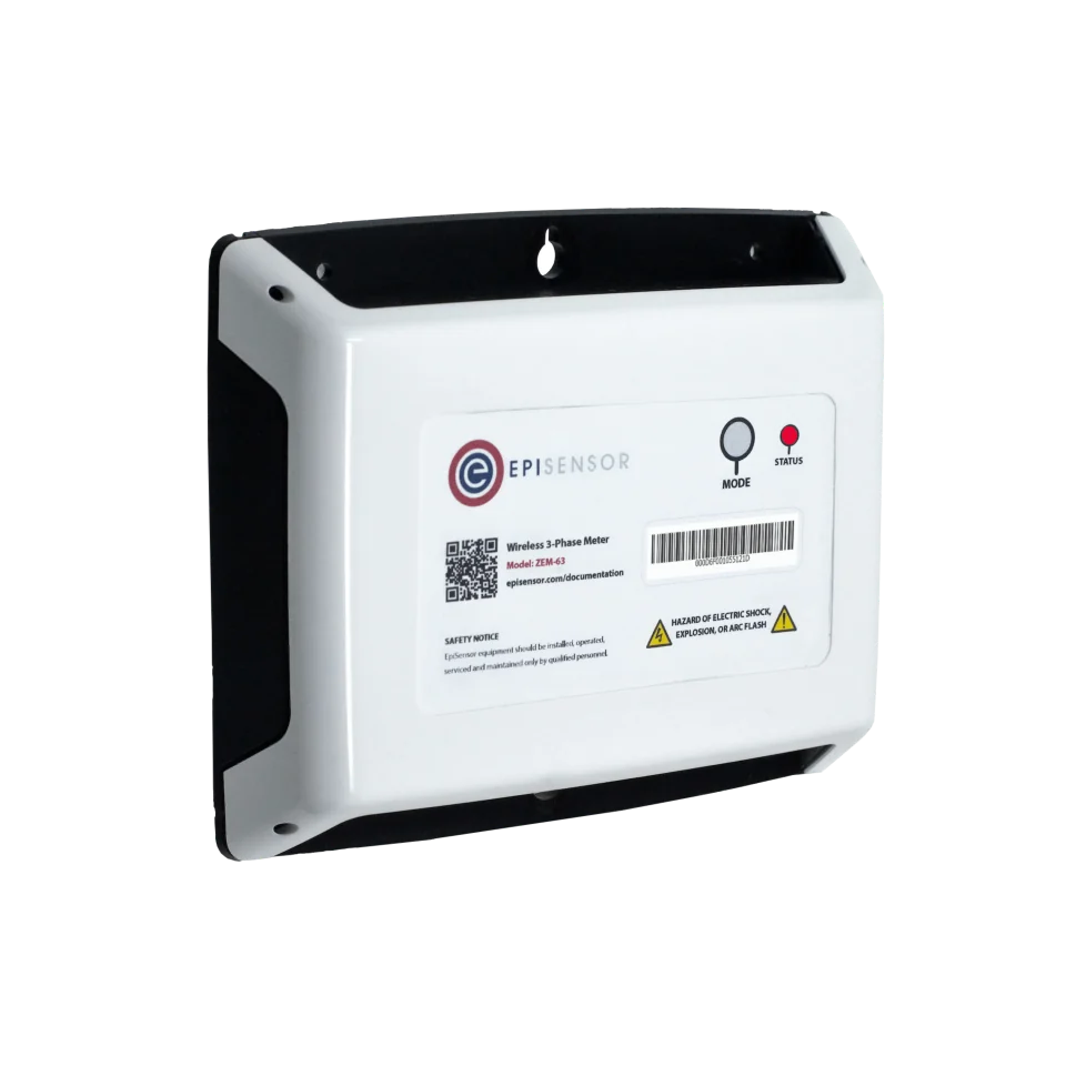
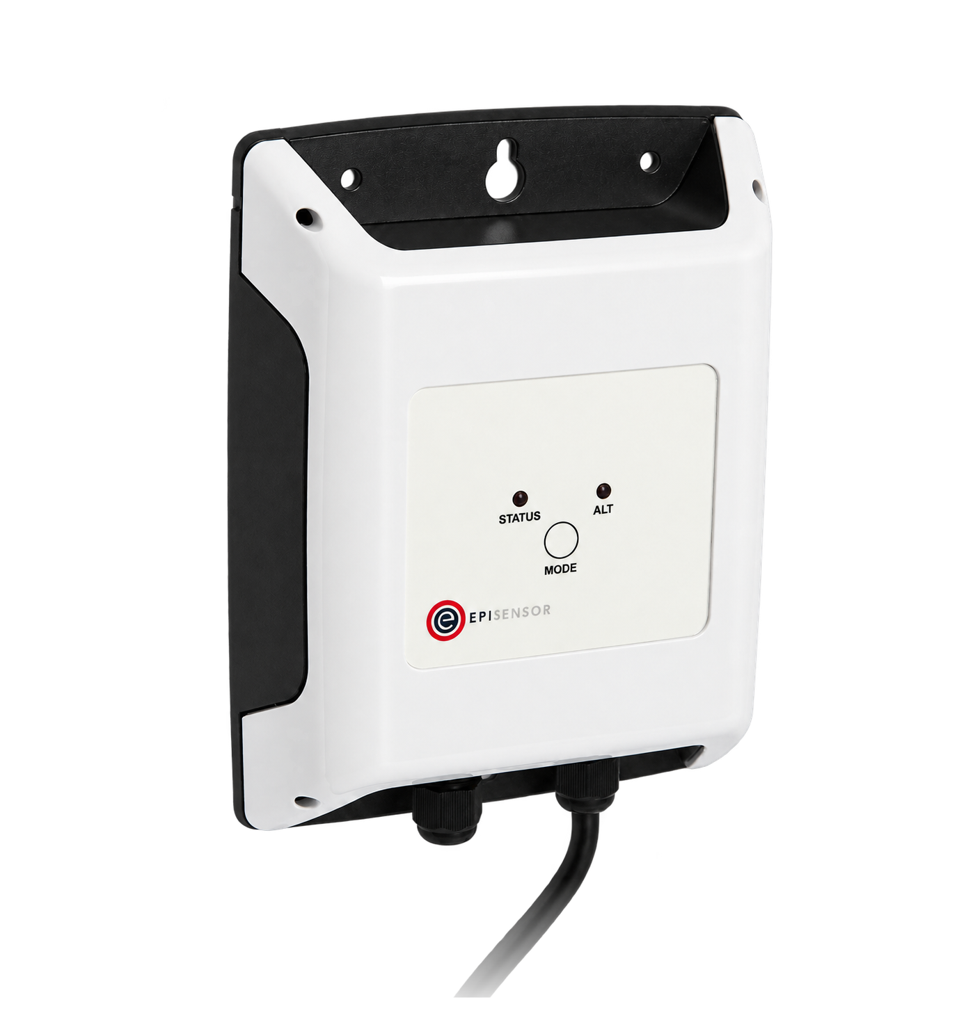
A ZEM measures the pump motor’s electrical input, and a ZIO reads flow and pressure transmitters, so the saving the affinity laws predict can be checked against measured data.